Wolves And Rabbits
December 1, 2009
 There are two general approaches to the solution of differential equations: analytical and numerical; since we are programmers, not mathematicians, we choose the numerical methods, which are easy but prone to divergence.
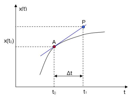
The Swiss mathematician Leonhard Euler, working at the great universities in Saint Petersburg and Berlin in the 1700s, developed the basic method: starting from the initial points, calculate the derivative (the tangent line) at each point and extrapolate the next point on the curve assuming that it is a straight line. The calculation of the derivative of a curve at point A, showing the predicted point at P, is illustrated at right. If the time interval is small enough, the difference between the predicted point and the actual point will be negligible.
A better method, developed by the German mathematicians Carl Runge and Martin Kutta around the year 1900, uses Euler’s method to extrapolate the mid-point of the time interval, then repeats Euler’s method, calculating the derivative of the extrapolated mid-point and extrapoliting to the end-point of the time interval; this is the second-order Runge-Kutta method. The most common method is the fourth-order Runge-Kutta method, as described in the Example of the R5RS Scheme Report, but the second-order method is good enough for our example. Here it is:
(define (wolves-rabbits init-rabbit rabbit-growth rabbit-death

                        init-wolf wolf-growth wolf-death limit)

  (let loop ((ts (list 0)) (rs (list init-rabbit)) (ws (list init-wolf)))

    (if (= (car ts) limit)

        (apply zip (map reverse (list ts rs ws)))

        (let* ((rabbit-deriv

                 (- (* rabbit-growth (car rs))

                    (* rabbit-death (car rs) (car ws))))

               (wolf-deriv

                 (- (* wolf-growth (car ws) (car rs))

                    (* wolf-death (car ws))))

               (rabbit-half

                 (+ (car rs) (/ rabbit-deriv 2)))

               (wolf-half

                 (+ (car ws) (/ wolf-deriv 2)))

               (rabbit-half-deriv

                 (- (* rabbit-growth rabbit-half)

                    (* rabbit-death rabbit-half wolf-half)))

               (wolf-half-deriv

                 (- (* wolf-growth wolf-half rabbit-half)

                    (* wolf-death wolf-half))))

          (loop (cons (+ (car ts) 1) ts)

                (cons (+ (car rs) rabbit-half-deriv) rs)

                (cons (+ (car ws) wolf-half-deriv) ws))))))
We use zip from the Standard Prelude. Here’s an example:
> (wolves-rabbits 40 15 0.1 0.01 0.005 0.1 5)

((0 40 15) (1 37.7575 16.49625)

  (2 35.11682084652719 17.920285997048907)

  (3 32.21720532523942 19.196647945977375)

  (4 29.21033531051106 20.25857350383283)

  (5 26.23820534547707 21.057736744807745))
You can run the simulation yourself at http://programmingpraxis.codepad.org/WXb79n5K.

My Haskell solution (see http://bonsaicode.wordpress.com/2009/12/01/programming-praxis-wolves-and-rabbits/ for a version with comments):
pops :: Fractional a => a -> a -> a -> a -> a -> a -> [(a, a)] pops r w rg wg rd wd = (r, w) : pops r' w' rg wg rd wd where dr x y = rg*x - rd*x*y dw x y = wg*x*y - wd*x rh = r + dr r w / 2 wh = w + dw w r / 2 r' = r + dr rh wh w' = w + dw wh rhThe reason, if you are curious, that the Runge-Kutta example appears in the Scheme reports is that it appeared in the Algol 60 report (which is also responsible for the title template “Revised^N Report on the Algorithmic Language X”, though neither Algol 60 nor Algol 68 never got beyond Revised^1).
The Algol 60 version is no beauty by modern standards, but here it is for comparison:
procedure RK (x,y,n,FKT,eps,eta,xE,yE,fi); value x,y; integer n;
Boolean fi; real x,eps,eta,xE; array y,yE; procedure FKT;
comment RK integrates the system y’k=fk(x,y1,y2,…,yn)(k=1,2,…n)
of differential equations with the method of Runge-Kutta with automatic
search for appropriate length of integration step. Parameters are: The
initial values x and y[k] for x and the unknown functions yk(x). The
order n of the system. The procedure FKT(x,y,n,z) which represents the
system to be integrated, i.e. the set of functions fk. The tolerance values eps
and eta which govern the accuracy of the numerical integration. The end
of the integration interval xE; The output parameter yE which represents
the solution x=xE. The Boolean variable fi, which must always be given
the value true for an isolated or first entry into RK. If however the functions
y must be available at several meshpoints x0,x1,…,xn, then the procedure
must be called repeatedly (with x=xk, xE=x(k+1), for k=0,1,…,n-1)
and then the later calls may occur with fi=false which saves computing
time. The input parameters of FKT must be x,y,z,n, the output parameter z
represents the set of derivatives z[k]=fk(x,y[1],y[2],…,y[n]) for x and
the actual y’s. A procedure comp enters as a non-local identifier;
begin
array z,y1,y2,y3[1:n]; real x1,x2,x3,H; Boolean out;
integer k,j; own real s,Hs;
procedure RK1ST (x,y,h,xe,ye); real x,h,xe; array y,ye;
comment RK1ST integrates one single Runge-Kutta step with
initial values x, y[k] which yields the output parameters xe=x+h
and ye[k], the latter being the solution at xe. Important: the
parameters n, FKT, z enter RK1ST as nonlocal entities;
begin
array w[1:n], a[1:5]; integer k,j;
a[1]:=a[2]:=a[5]:=h/2; a[3]:=a[4]:=h;
xe:=x;
for k:=1 step 1 until n do ye[k]:=w[k]:=y[k];
for j:=1 step 1 until 4 do
begin
FKT(xe,w,n,z);
xe:=x+a[j];
for k:=1 step 1 until n do
begin
w[k]:=y[k]+a[j]TIMESz[k];
ye[k]:=ye[k]+a[j+1]TIMESz[k]/3
end k
end j
end RK1ST;
Begin of program:
if fi then begin H:=xE-x; s:=0 end else H:=Hs;
out:=false;
AA: if (x+2.01TIMESH-xE)>0) EQUIVALENCE (H>0) then
begin Hs:=H; out:=true; H:=(xE-x)/2 end if;
RK1ST (x,y,2TIMESH,x1,y1);
BB: RK1ST (x,y,H,x2,y2); RK1ST (x2,y2,H,x3,y3);
for k:=1 step 1 until n do
if comp (y1[k],y3[k],eta)>eps then goto CC;
comment comp(a,b,c) is a function designator, the value of
which is the absolute value of the difference of the mantissae of a
and b, after the exponents of these quantities have been made equal
to the largest of the exponents of the originally given parameters
a, b, c;
x:=x3; if out then goto DD;
for k:=1 step 1 until n do y[k]:=y3[k];
if s=5 then begin s:=0; H:=2TIMESH end if;
s:=s+1; goto AA;
CC: H:=0.5TIMESX; out:=false; x1:=x2;
for k:=1 step 1 until n do y1[k]:=y2[k];
goto BB;
DD: for k:=1 step 1 until n do yE[k]:=y3[k]
end RK
Arrgh, indentation lost. Well, you can read it at http://www.masswerk.at/algol60/report.htm .
I must admit that I cheated a tiny bit. I took a stare at your Haskell solution, and basically did a straightforward port to Python (my “just muck around” language of choice for tiny problems like that). I used generators in lieu of laziness, but other than that, you should recognize it. It’s been quite some time since I had to implement Runge-Kutta integrators (the most recent application of this kind of stuff that I’ve done would have been simple particle systems where just Euler steps are okay for most of my purposes) so it was a nice review.
Anyway, here’s the code:
#!/usr/bin/env python # https://programmingpraxis.com/2009/12/01/wolves-and-rabbits/ def population(r, w, rg, wg, rd, wd): def dr(x, y): return rg * x - rd * x * y def dw(x, y): return wg * x * y - wd * x while True: yield r, w rh = r + dr(r, w) / 2. wh = w + dw(w, r) / 2. r = r + dr(rh, wh) w = w + dw(wh, rh) g = population(40, 15, 0.1, 0.005, 0.01, 0.1) for x in range(201): r, w = g.next() print r, w[…] […]
here’s some Matlab code to solve the problem using the 2nd order Runge-Kutta
you can use a variable time step if you like (deltaT)
function [t, wolves, rabbits]=rkWR(R0, W0, Rg, Wg, Rd, Wd, deltaT, maxT )
h=deltaT;
tmax= maxT;
t=0:h:tmax;
nsteps = tmax/h;
wolves = zeros(nsteps+1,1);
rabbits = zeros(nsteps+1,1);
wolves(1)=W0;
rabbits(1)=R0;
for i=1:nsteps;
rk1 = h*rabbitsFunc(Rg,Rd, rabbits(i), wolves(i));
wk1 = h*wolvesFunc(Wg,Wd, rabbits(i), wolves(i));
rk2 = h*rabbitsFunc(Rg,Rd, rabbits(i)+rk1/2, wolves(i)+wk1/2);
wk2 = h*wolvesFunc(Wg,Wd, rabbits(i)+rk1/2, wolves(i)+wk1/2);
rabbits(i+1)=rabbits(i)+rk2;
wolves(i+1)=wolves(i)+wk2;
end
end
function [dWdt] = rabbitsFunc(Rg, Rd, R, W )
dWdt =Rg*R-Rd*R*W;
end
function [dRdt] = wolvesFunc(Wg, Wd, R, W)
dRdt = Wg*R*W-Wd*W;
end
to run for this example
[t,w,r] = rkWR(40, 15, 0.1, 0.005, 0.01, 0.1,1, 200);
figure, plot(t, w,’-+r’);
hold on, plot(t, r, ‘-ob’);