Integer Factorization
April 30, 2010
We have now discussed several different factorization algorithms: trial division, wheel factorization, Fermat’s method, Pollard’s rho method, Pollard’s p-1 method in both one-stage and two-stage variants, and the elliptic curve method in both one–stage and two–stage variants. So, if you must factor a large integer, where do you start?
The basic idea is to perform several methods, starting with simple methods and working up to more complicated ones until the factorization is determined. The exact choice of the methods to be used and the decision on when to abandon one method in favor of another is idiosyncratic at best. There are many possibilities, and many degrees of freedom, that suggest one alternative or another.
Your task is to write a program that factors large integers using some mix of the factorization methods we have studied. When you are finished, you are welcome to read or run a suggested solution, or to post your own solution or discuss the exercise in the comments below.
Modern Elliptic Curve Factorization, Part 2
April 27, 2010
The elliptic curve factorization algorithm is remarkably similar to Pollard’s p-1 algorithm:
define p-1(n, B1, B2)
|
1 |
define ecf(n, B1, B2, C)
|
| q = 2 | 2 | Qx,z ∈ C // random point |
| for p ∈ π(2 … B1) | 3 | for p ∈ π(2 … B1) |
a = ⌊logp B1⌋
|
4 |
a = ⌊logp B1⌋
|
q = qpa (mod n)
|
5 | Q = pa ⊗C Q |
g = gcd(q, n)
|
6 |
g = gcd(Qz, n)
|
| if (1 < g < n) return g | 7 | if (1 < g < n) return g |
| for p ∈ π(B1 … B2) | 8 | for p ∈ π(B1 … B2) |
q = qp (mod n)
|
9 | Q = p ⊗C Q |
| 10 |
g = g × Qz (mod n)
|
|
g = gcd(q, n)
|
11 |
g = gcd(g, n)
|
| if (1 < g < n) return g | 12 | if (1 < g < n) return g |
| return failure | 13 | return failure |
Lines 3 and 8 loop over the same lists of primes. Line 4 computes the same maximum exponent. Lines 6 and 7, and lines 11 and 12, compute the same greatest common divisor. And line 13 returns the same failure. The structures of the two algorithms are identical. Also, note that both algorithms use variables that retain their meaning from the first stage (lines 2 to 7) to the second stage (lines 8 to 12).
Lines 2, 5, 9 and 10 differ because p-1 is based on modular arithmetic and ecf is based on elliptic arithmetic (note that the ⊗C operator, otimes-sub-C, indicates elliptic multiplication on curve C). The most important difference is on the first line, where ecf has an extra argument C indicating the choice of elliptic curve. If the p-1 method fails, there is nothing to do, but if the ecf method fails, you can try again with a different curve.
Use of Montgomery’s elliptic curve parameterization from the previous exercise is a huge benefit. Lenstra’s original algorithm, which is the first stage of the modern algorithm, required that we check the greatest common divisor at each step, looking for a failure of the elliptic arithmetic. With the modern algorithm, we compute the greatest common divisor only once, at the end, because Montgomery’s parameterization has the property that a failure of the elliptic arithmetic propagates through the calculation. And without inversions, Montgomery’s parameterization is also much faster to calculate. Brent’s parameterization of the randomly-selected curve is also important, as it guarantees that the order of the curve (the number of points) will be a multiple of 12, which has various good mathematical properties that we won’t enumerate here.
There is a simple coding trick that can speed up the second stage. Instead of multiplying each prime times Q, we iterate over i from B1 + 1 to B2, adding 2Q at each step; when i is prime, the current Q can be accumulated into the running solution. Again, we defer the calculation of the greatest common divisor until the end of the iteration.
Your task is to write a function that performs elliptic curve factorization. When you are finished, you are welcome to read or run a suggested solution, or to post your own solution or discuss the exercise in the comments below.
Modern Elliptic Curve Factorization, Part 1
April 23, 2010
We discussed Hendrik Lenstra’s algorithm for factoring integers using elliptic curves in three previous exercises. After Lenstra published his algorithm in 1987, mathematicians studied the algorithm extensively and made many improvements. In this exercise, and the next, we will study a two-stage version of elliptic curve factorization that features improved elliptic arithmetic and is much faster than Lenstra’s original algorithm. Today’s exercise looks at the improved elliptic arithmetic; we will look at the two-stage algorithm in the next exercise.
If you look at Lenstra’s original algorithm, much of the time is spent calculating modular inverses. Peter Montgomery worked out a way to eliminate the modular inverses by changing the elliptic arithmetic; instead of using the curve y2 = x3 + ax + b, Montgomery uses the curve y2 = x3 + ax2 + x. Additionally, he does a co-ordinate transform to eliminate the y variable, so we don’t need to figure out which of the quadratic roots to follow. Finally, Montgomery stores the numerator and denominator of the a parameter separately, eliminating the modular inverse. We won’t give more of the math; for those who are interested, a good reference is Prime Numbers: A Computational Perspective by Richard Crandall and Carl Pomerance.
Here are the elliptic addition, doubling and multiplication rules for Montgomery’s elliptic curves:
A curve is given by the formula y2 = x3 + (An / Ad – 2)x2 + x (mod n).
A point is stored as a two-tuple containing its x and z co-ordinates.
To add two points P1(x1,z1) and P2(x2,z2), given the point P0(x0,z0) = P1 – P2 (notice that the curve is not used in the calculation):
x = ((x1–z1) × (x2+z2) + (x1+z1) × (x2–z2))2 × z0 mod n
z = ((x1–z1) × (x2+z2) – (x1+z1) × (x2–z2))2 × x0 mod nTo double the point P:
x = (x+z)2 × (x–z)2 × 4 × Ad mod n
z = (4 × Ad × (x–z)2 + t × An) × t mod n where t = (x+z)2 – (x–z)2Multiplication is done by an adding/doubling ladder, similar to the method used in the Lucas chain in the exercise on the Baillie-Wagstaff primality checker; the Lucas chain is needed so that we always have the point P1–P2. For instance, the product 13P is done by the following ladder:
2P = double(P)
3P = add(2P, P, P)
4P = double(2P)
6P = double(3P)
7P = add(4P, 3P, P)
13P = add(7P, 6P, P)
Richard Brent gave a method to find a suitable elliptic curve and a point on the curve given an initial seed s on the half-open range [6, n), with all operations done modulo n:
u = s2 – 5
v = 4sAn = (v–u)3 (3u+v)
Ad = 4u3vP = (u3, v3)
Your task today is to write the three functions that add, double, and multiply points on an elliptic curve and the function that finds a curve and a point on the curve; the payoff will be in the next exercise that presents elliptic curve factorization. When you are finished, you are welcome to read or run a suggested solution, or to post your own solution or discuss the exercise in the comments below.
145 Puzzle
April 20, 2010
Consider this math puzzle:
Form all the arithmetic expressions that consist of the digits one through nine, in order, with a plus-sign, a times-sign, or a null character interpolated between each pair of digits; for instance, 12+34*56+7*89 is a valid expression that evaluates to 2539. What number is the most frequent result of evaluating all possible arithmetic expressions formed as described above? How many times does it occur? What are the expressions that evaluate to that result?
Your task is to answer the three questions. When you are finished, you are welcome to read or run a suggested solution, or to post your own solution or discuss the exercise in the comments below.
Expression Evaluation
April 16, 2010
The very first exercise at Programming Praxis evaluated expressions given in reverse-polish notation. In today’s exercise, we write a function to evaluate expressions given as strings in the normal infix notation; for instance, given the string “12 * (34 + 56)”, the function returns the number 1080. We do this by writing a parser for the following grammar:
| expr | → | term |
| expr + term | ||
| expr – term | ||
| term | → | fact |
| term * fact | ||
| term / fact | ||
| fact | → | numb |
| ( expr ) |
The grammar specifies the syntax of the language; it is up to the program to provide the semantics. Note that the grammar handles the precedences and associativities of the operators. For example, since expressions are made up from terms, multiplication and division are processed before addition and subtraction.
The normal algorithm used to parse expressions is called recursive-descent parsing because a series of mutually-recursive functions, one per grammar element, call each other, starting from the top-level grammar element (in our case, expr) and descending until the beginning of the string being parsed can be identified, whereupon the recursion goes back up the chain of mutually-recursive functions until the next part of the string can be parsed, and so on, up and down the chain until the end of the string is reached, all the time accumulating the value of the expression.
Your task is to write a function that evaluates expressions according to the grammar given above. When you are finished, you are welcome to read or run a suggested solution, or to post your own solution or discuss the exercise in the comments below.
Traveling Salesman: Minimum Spanning Tree
April 13, 2010
We looked at the traveling salesman problem in two previous exercises. We also studied two algorithms for computing the minimum spanning tree. In today’s exercise, we will use a minimum spanning tree as the basis for computing a traveling salesman tour.
It is easy to convert a minimum spanning tree to a traveling salesman tour. Pick a starting vertex on the minimum spanning tree; any one will do. Then perform depth-first search on the tree rooted at the selected vertex, adding each vertex to the traveling salesman tour as it is selected. The resulting tour is guaranteed to be no longer than twice the optimal tour. Considering the speed of the algorithm, that’s a pretty good result.
Your task is to write a program that finds traveling salesman solutions using a minimum spanning tree as described above. When you are finished, you are welcome to read or run a suggested solution, or to post your own solution or discuss the exercise in the comments below.
Minimum Spanning Tree: Prim’s Algorithm
April 9, 2010
 In the previous exercise we studied Kruskal’s algorithm for computing the minimum spanning tree of a weighted graph. Today we study an algorithm developed in 1930 by the Czech mathematician Vojtěch Jarník and rediscovered by Robert Prim in 1957.
Kruskal’s algorithm works by creating a singleton tree for each vertex and merging the trees by taking at each step the minimum-weight edge that joins two trees. Prim’s algorithm is the opposite; it starts with a single vertex and repeatedly joins the minimum-weight edge that joins the tree to a non-tree vertex. At each step the tree is a minimum spanning tree of the vertices that have been processed thus far.
Your task is to write a program to find the minimum spanning tree of a graph using Prim’s algorithm. When you are finished, you are welcome to read or run a suggested solution, or to post your own solution or discuss the exercise in the comments below.
Minimum Spanning Tree: Kruskal’s Algorithm
April 6, 2010
We studied disjoint sets in the previous exercise. In today’s exercise we use disjoint sets to implement Kruskal’s algorithm to find the minimum spanning tree of a graph.
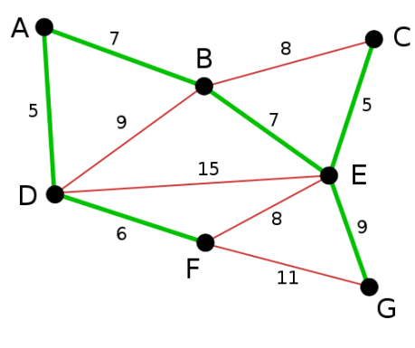
A graph is a generalized tree in which vertices may be connected by edges in any configuration. Edges may be directed (from one vertex to another) or undirected, and may be weighted or unweighted. On an undirected weighted graph, a spanning tree is a collection of edges that connects all vertices, and a minimum spanning tree has the lowest total edge-weight of all possible spanning trees. A minimum spanning tree always has one less edge than there are vertices in the graph.
Joseph Kruskal developed the following algorithm for determining the minimum spanning tree in 1956, where V is the set of vertices and E is the set of weighted edges:
- Create a disjoint set in which each vertex is a singleton partition.
- Loop over the edges in order by increasing weight
- If the current edge connects two unconnected partitions
- Add the edge to the minimum spanning tree
- Merge the two partitions
- If the spanning tree is complete, return it, otherwise go to the next-larger edge
Your task is to write a program that implements Kruskal’s algorithm. When you are finished, you are welcome to read or run a suggested solution, or to post your own solution or discuss the exercise in the comments below.
Disjoint Sets
April 2, 2010
 Disjoint sets are a data structure that supports grouping, or partitioning, n distinct elements into a collection of sets, each containing a distinct subset of the elements. The operations supported by the data structure are find, which determines to which subset a particular element belongs, and union, when merges two subsets into one.
It is straight forward to implement disjoint sets using linked lists. The problem is that such a representation can have quadratic performance in the worst case, and the worst case, or something close to it, occurs reasonably often.
Thus, most algorithms textbooks describe a data structure called a disjoint-set forest. Each subset is represented by a tree, with each node containing a pointer to its parent; these are generalized trees, not binary trees, with potentially many children at each node. The make-set function returns a singleton tree, find chases parent pointers to the root of the tree, and union makes the root of one of the trees point to the root of the other in its parent. Two heuristics are common; union joins the tree with smaller rank (the upper bound on the depth of the tree) as a sub-tree to the tree with greater rank, and path compression replaces the parent pointer of each node with a pointer to the root of the tree instead of a pointer to the parent.
Your task is to implement a library that provides the make-set, find and union operations for disjoint sets, using the disjoint-set forest data structure described above. When you are finished, you are welcome to read or run a suggested solution, or to post your own solution or discuss the exercise in the comments below.
