Programming Praxis

We wrote a basic library of AVL tree functions in the previous exercise. In today’s exercise we will extend the library with the following functions:

size – Return the number of items in an input tree.

nth – Return the nth item in an input tree, or an error if n is out of range.

rank – Return the ordinal position of a key in an input tree, or an error if the key is not present in the tree.

map – Return a tree with all of the values in an input tree replaced by the results of an input function that takes an existing key and value; the keys of the tree are unchanged.

fold – Return a single value obtained by evaluating a given procedure at each node of the tree, in order. The procedure takes three parameters: the current key, the associated value, and a base value that accumulates the results of previous evaluations of the procedure. Returns the accumulated value after all nodes of the tree have been considered.

for-each – Evaluate a given procedure at each node of the tree, in order. The procedure takes two parameters: the current key and the associated value. Returns nothing; the procedure is evaluated only for its side effects.

to-tree – Return a tree containing the key/value pairs of an input list.

Your task is to add the functions described above to the AVL tree library of the previous exercise. When you are finished, you are welcome to read or run a suggested solution, or to post your own solution or discuss the exercise in the comments below.

Pages: 1 2

In past exercises we have seen several flavors of search trees: simple (unbalanced) binary trees, red/black trees, treaps, and ternary search trees. In today’s exercise we look at the oldest, and in some ways simplest, of the balanced binary search trees, known as AVL trees, invented in 1962 by the Russian mathematicians Georgii Maksimovich Adelson-Velskii and Evgenii Mikhailovich Landis.

AVL trees are a type of binary search tree, and maintain the property that all elements in the left child of each node have keys that are less than the key of the current node, and all elements in the right child of each node have keys that are greater than the key of the current node. AVL trees maintain balance using a height field in each node, along with the key, value, and pointers to the two children; the height of a node is length of the longest path from the node to the bottom of the tree. An AVL tree is balanced if, for every node in the tree, the heights of its children differ by no more than 1. Thus, the maximum height of the tree is O(log₂ n), where n is the number of nodes in the tree, so all operations — lookup, insert and delete — can be performed in guaranteed (not expected, not amortized) logarithmic time in both the average case and the worst case.

The lookup operation is simple, and works exactly the same way as a simple (unbalanced) binary search tree. If the key at the root of the tree is the desired key, return the associated value. Otherwise, lookup the desired key recursively in either the left subtree or the right subtree, depending on whether the desired key is less than or greater than the current tree. If you reach a nil tree, the key is not in the tree and the search fails.

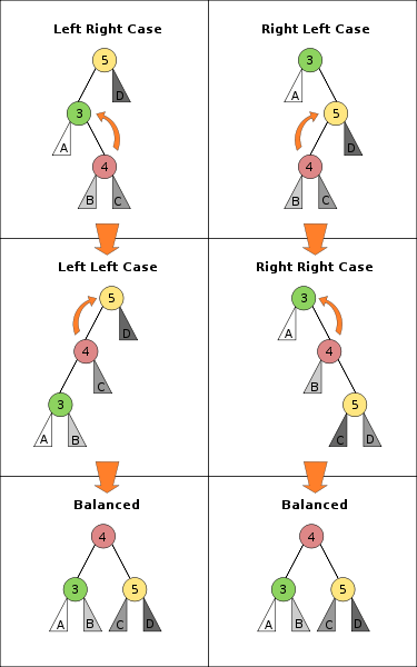
The insertion operation works by searching to the point where the new node is to be inserted, then rewriting the tree locally to insert the new point. This maintains the binary search tree property that all left children are less than the current node and all right children are greater than the current but may violate the AVL tree property that the height of the two children of a node differ by no more than 1. In that case, either one or two local rotations are performed to maintain the binary search tree property and regain the AVL tree property; the box at right, which is stolen from Wikipedia, gives the two symmetric cases. There are two special cases, where insertion occurs at the leaf of a tree, and where the key already exists in the tree; be sure to handle them properly.

As is usual with tree operations, deletion is the trickiest operation. The basic idea is to search to the node to be deleted, replace it with either its maximal predecessor or minimal successor, then delete the maximal predecessor or minimal successor and rebalance the tree at each node back up to the point of the replacement. In the normal case, only a few rebalancing operations are required, as there is sufficient slack in the tree to absorb any imbalance. Note that although this description sounds simple, getting the details right can be anything but. There is a single special case: when the key doesn’t exist in the tree, the original tree should be returned.

The final operation we consider enrolls the elements of an AVL tree in a list, in order. The procedure begins at the root of the tree and recursively appends the list formed by the left child, the current item, and the list formed by the right child; the base of the recursion is the nil tree, which is represented as a null list.

Your task is to write a library of functions for manipulating AVL trees; be sure to provide a comprehensive test suite. When you are finished, you are welcome to read or run a suggested solution, or to post your own solution or discuss the exercise in the comments below.

Pages: 1 2

The RSA encryption algorithm, which we studied in a previous exercise, relies on the difficulty of factoring large integers for its security. Another cryptosystem was developed by Michael Rabin about the same time that Rivest, Shamir and Adelman were developing RSA, and is also based on the difficulty of factoring large integers. Although it is theoretically stronger than RSA, Rabin’s cryptosystem never became popular because in practice RSA is about equally strong, because RSA was first by about a year, and because Rabin’s cryptosystem requires additional work to disambiguate the decryption.

Rabin’s cryptosystem is based on two integers p and q each congruent to 3 modulo 4 which form the private key; their product, n = p × q, is the public key. Then to encrypt the message m, the ciphertext is c = m² mod n. The plaintext is recovered by finding the four square roots of c modulo m, and choosing the correct message from the four possibilities. Note that a text message is converted to a number m in the same way as RSA.

The four square roots of the ciphertext c are calculated as follows. First determine a and b satisfying the equation a × p + b × q = 1 using the extended euclidean algorithm of a prior exercise. Compute r = c^(p+1)/4 mod p. Compute s = c^(q+1)/4 mod q. Compute x = (a × p × s + b × q × r) mod n. Compute y = (a × p × s − b × q × r) mod n. Then the four square roots are m₁ = x, m₂ = −x, m₃ = y, and m₄ = −y.

The problem with Rabin’s cryptosystem is the decryption into four possible messages. The solution is to pad the message in such a way that only one of the four possible messages fits the padding. This is done by replicating the bits of the last portion of the message, adding them to the end of the message; only the correct decryption will have the trailing bits duplicated.

An example makes this clear. Consider p = 7, q = 11, and n = 77. By the euclidean algorithm, (−3)×7 + 2×11 = 1, so a = −3 and b = 2. Now we send the message 5₁₀ = 101₂, padded to the message m = 101101₂ = 45₁₀. The ciphertext is c = 45² mod 77 = 23. Decryption first computes r = 23² mod 7 = 4 and s = 23² mod 11 = 1. Then x = (−3)×7×1 + 2×11×4 mod 77 = 67 and y = (−3)×7×1 − 2×11×4 mod 77 = 45. Thus two of the square roots are 67 and 45, and the other two are 77 − 67 = 10 and 77 − 45 = 32. Now 10₁₀ = 001010₂, 32₁₀ = 100000₂, 45₁₀ = 101101₂ and 67₁₀ = 1000011₂, so only 101101₂ has the required redundancy and the payload is 101₂ = 5₁₀.

In normal usage, the Rabin cryptosystem is generally based on blocks of 512 bits, or 1024 bits, or 2048 bits, of which the last 64 bits consist of padding, giving a payload of 448, 960 or 1984 bits (56, 120 or 248 bytes), respectively; sometimes a padding of 128 bits is used, if there is some concern about the (very unlikely) possibility of a false duplicate. Another method that is sometimes used pads the message with 64 0-bits (or 128 bits instead of 64 bits, or 1-bits instead of 0-bits, or some other known pattern), so that only the square root with the desired pattern is used. The message is split into blocks of the needed size, and is extended by adding a 1-bit followed by as many 0-bits as are needed to make the message a multiple of the block length.

Your task is to write functions that generate keys and encrypt and decrypt messages using the Rabin cryptosystem. When you are finished, you are welcome to read or run a suggested solution, or to post your own solution or discuss the exercise in the comments below.

Pages: 1 2

Two weeks ago, on November 5th, the ACM sponsored its 2011 Mid-Central Regional Programming Contest for college student programmers. The seven problems, which were to be solved in five hours by teams of three programmers with a single shared computer, have been published. Today’s exercise asks you to solve the first problem involving grade school multiplication:

An educational software company, All Computer Math (ACM), has a section on multiplication of integers. They want to display the calculations in the traditional grade school format, like the following computation of 432 × 5678:

    432
   5678
-------
   3456
  3024
 2592
2160
-------
2452896

Note well that the final product is printed without any leading spaces, but that leading spaces are necessary on some of the other lines to maintain proper alignment. However, as per our regional rules, there should never be any lines with trailing white space. Note that the lines of dashes have length matching the final product.

As a special case, when one of the digits of the second operand is a zero, it generates a single 0 in the partial answers, and the next partial result should be on the same line rather than the next line down. For example, consider the following product of 200001 × 90040:

     200001
      90040
-----------
    8000040
180000900
-----------
18008090040

The rightmost digit of the second operand is a 0, causing a 0 to be placed in the rightmost column of the first partial product. However, rather than continue to a new line, the partial product of 4 × 200001 is placed on the same line as that 0. The third and fourth least-significant digits of the second operand are zeros, each resulting in a 0 in the second partial product on the same line as the result of 9 × 200001.

As a final special case, if there is only one line in the partial answer, it constitutes a full answer, and so there is no need for computing a sum. For example, a computation of 246 × 70 would be formatted as

  246
   70
-----
17220

Your job is to generate the solution displays.

Input: The input contains one or more data sets. Each data set consists of two positive integers on a line, designating the operands in the desired order. Neither number will have more than 6 digits, and neither will have leading zeros. After the last data set is a line containing only 0 0.

Output: For each data set, output a label line containing “Problem ” with the number of the problem, followed by the complete multiplication problem in accordance with the format rules described above.

Warning: A standard int type cannot properly handle 12-digit numbers. You should use a 64-bit type (i.e., a long in Java, or a long long in C++).

Example Input:	Example Output:
432 5678 200001 90040 246 70 0 0	Problem 1     432    5678 -------    3456   3024  2592 2160 ------- 2452896 Problem 2      200001       90040 -----------     8000040 180000900 ----------- 18008090040 Problem 3   246    70 ----- 17220

Your task is to solve Problem A. When you are finished, you are welcome to read or run a suggested solution, or to post your own solution or discuss the exercise in the comments below. As a special added bonus, feel free to solve any of the other problems in the programming contest, and to post your solution in the comments below.

Pages: 1 2

Today’s exercise comes to us from Michi’s blog:

Phil Harvey wants us to partition {1,…,16} into two sets of equal size so each subset has the same sum, sum of squares and sum of cubes.

Your task is to find the partition. When you are finished, you are welcome to read or run a suggested solution, or to post your own solution or discuss the exercise in the comments below.

Pages: 1 2

A recent exercise generated (sorry) a discussion of generators in the comments, so in today’s exercise we will take a look at generators. The recent exercise that used a priority queue in place of the array in the Sieve of Eratosthenes works well with generators; in fact, Mike’s contributed solution used a Python generator.

Your task is to rewrite the prime number generator of the previous exercise to return primes using a generator instead of a list. When you are finished, you are welcome to read or run a suggested solution, or to post your own solution or discuss the exercise in the comments below.

Pages: 1 2

We recently examined an improved second stage for John Pollard’s p−1 factoring algorithm. In today’s exercise we will look at the similar second stage for the elliptic curve factoring algorithm, an optimization known as the improved standard continuation. We will be following Algorithm 7.4.4 in the book Prime Numbers: A Computational Perspective by Richard Crandall and Carl Pomerance.

Recall from our previous exercises that the first stage of the elliptic curve algorithm ends with a point Q that fails to find a factor. In the second stage we want to calculate elliptic multiples of Q: 2Q, 4Q, 6Q, and so on. Recall also that the p−1 method uses a strength reduction technique to replace exponentiation with multiplication. The improved standard continuation uses a similar technique to reduce elliptic multiplication, which is slow, to two modular multiplications plus an occasional elliptic addition. Here is the algorithm as given by Crandall and Pomerance:

S₁ = doubleh(Q)
S₂ = doubleh(S₁)
for (d ∈ [1,D]) { // this loop computes S_d = [2d]Q
    if (d > 2) S_d = addh(S_d−1, S₁, S_d−2)
    β_d = X(S_d) Z(S_d) (mod n)
}
g = 1
B = B₁ − 1 // B is odd
T = [B − 2D]Q // via Algorithm 7.2.7
R = B[Q] // via Algorithm 7.2.7
for (r = B; r < B₂; r = r + 2D) {
    α = X(R) Z(R) mod n
    for (prime q ∈ [r + 2, r + 2D]) { // loop over primes
        δ = (q − r) / 2 // distance to next prime
        g = g((X[R] − X(S_δ))(Z(R) + Z(S_δ)) − α + β_δ) mod n
    }
    (R, T) = (addh(R, S_D, T), R)
}
g = gcd(g, n)
if (1 < g < n) return g // found a nontrivial factor of n

In the notation of Crandall and Pomerance, B₁ is the first-stage bound and B₂ is the second-stage bound. D is a parameter that mediates a time-space trade-off, with a larger D taking more space but running faster; the memory required is about 3D n-sized integers. Q, R and T are points on the elliptic curve; the coordinates of point P are X(P) and Z(P). S[1 .. D] is an array of elliptic points, and β[1 .. D] stores the products of the X and Z coordinates of the elliptic points in S.

The S array corresponds to the array that we used in the second stage of the p−1 algorithm, and is built at runtime in a similar way in the first loop (on d) of the algorithm given above. Then the primes from B₁ to B₂ are processed in segments of size 2D, with r the base value of each segment and R the corresponding elliptic point. At each prime in the segment the difference to the base of the segment is calculated, then the stored values of S_δ and β_δ are used to update the product g. When all the primes have been calculated, a single gcd is calculated; if it is nontrivial, it is reported, otherwise the curve has failed to find a factor and a different curve must be tried.

The long formula that updates g takes the place of the elliptic multiplications of the first stage, in a very clever way. If you have available points R and S[1 .. D], the elliptic multiplication [s]Q = [r + δ]Q = O can be tested by checking whether the cross product X_r Z_δ − X_δ Z_r has a nontrivial gcd with n; simple algebra can reduce the work of computing the cross product even further with the formula shown in the algorithm.

Thus, by storing precomputed values of X_δ, Z_δ and the product X_δ Z_δ, it is possible to loop through the primes from B₁ to B₂ with only two modular multiplications per prime, plus a single elliptical addition for each segment.

Your task is to write a function to compute factors using the improved standard continuation of the elliptic curve factorization method. When you are finished, you are welcome to read or run a suggested solution, or to post your own solution or discuss the exercise in the comments below.

Pages: 1 2 3

Craps is a gambling game played with two dice. The “shooter” begins the game by rolling two dice. If the pips on the dice total 2, 3 or 12, the shooter loses. If the pips on the dice total 7 or 11, the shooter wins. If the pips on the dice total 4, 5, 6, 8, 9, or 10, the total of the pips establishes the “point” and shooter continues to roll until he rolls the point, when he wins, or he rolls a 7, when he loses.

Your task is to write a program that simulates a game of craps. Use the program to calculate various statistics: What is the most common roll? What is the average winning percentage? What is the average number of rolls in a game? The maximum? Or you can make your own questions. When you are finished, you are welcome to read or run a suggested solution, or to post your own solution or discuss the exercise in the comments below.

Pages: 1 2

John McCarthy, the inventor of Lisp, died on October 23, 2011. In his honor we will implement a Lisp interpreter in today’s exercise. He first described Lisp in an academic paper, and the LISP 1.5 Programmer’s Manual, published in 1962 but still in print, is an early definition of the language (the LISP 1.0 manual by Patricia Fox was dated 1960, which is usually cited as the birth year of Lisp, even though Lisp was formally specified as early as 1958). McCarthy defines the eval/apply yin/yang that is at the heart of Lisp on page 13, in what Alan Kay described as the Maxwell’s equations of software. We begin with the definition of apply:

apply[fn;x;a] =
     [atom[fn] → [eq[fn;CAR] → caar[x];
                 eq[fn;CDR] → cdar[x];
                 eq[fn;CONS] → cons[car[x];cadr[x]];
                 eq[fn;ATOM] → atom[car[x]];
                 eq[fn;EQ] → eq[car[x];cadr[x]];
                 T → apply[eval[fn;a];x;a]];
     eq[car[fn];LAMBDA] → eval[caddr[fn]; pairlis[cadr[fn];x;a]];
     eq[car[fn];LABEL] → apply[caddr[fn];x;cons[cons[cadr[fn];caddr[fn]];a]]]

Apply interprets expressions. The first clause dispatches on the various built-in functions of Lisp, calling the underlying language (in this case, Lisp, since this is a meta-circular evaluator) to evaluate the function. The second clause evaluates functions defined by lambda by calling eval. The third clause is special; it evaluates recursive functions defined by label by first adding the function to the environment, then calling apply recursively to evaluate the new function. Apply uses an auxiliary function pairlis to insert function definitions in the environment a; as an example, pairlis[(A B C);(U V W);((D . X) (E . Y))] evaluates to ((A . U) (B . V) (C . W) (D . X) (E . Y)):

pairlis[x;y;a] = [null[x] → a; T → cons[cons[car[x];car[y]];
                 pairlis[cdr[x];cdr[y];a]]]

Eval handles statements, which are known as special forms in the parlance of Lisp. In a function, the elements of an expression are all evaluated before the function at the head of the expression is called, but in a statement the order of evaluation may change; for instance, in an if statement only one of the two consequents is evaluated. Here is eval:

eval[e;a] = [atom[e] → cdr[assoc[e;a]];
     atom[car[e]] →
             [eq[car[e];QUOTE] → cadr[e];
             eq[car[e];COND] → evcon[cdr[e];a];
             T → apply[car[e];evlis[cdr[e];a];a]];
     T → apply[car[e];evlis[cdr[e];a];a]]

Eval handles two special forms: Quote handles its argument literally rather than evaluating it as an expressions. Cond executes code conditionally, checking the predicate of each clause until it finds one that is true, when it evaluates the associated expression. Eval uses three auxiliary functions. The first is assoc, which performs a lookup in an environment; for instance, assoc[B;((A . (M N)), (B . (CAR X)), (C . (QUOTE M)), (C . (CDR X)))] evaluates to (B . (CAR X)):

assoc[x;a] = [equal[caar[a];x]→car[a]; T → assoc[x;cdr[a]]]

Evcon interprets a cond statement, evaluating the predicate of each clause, then evaluating the expression associated with the first predicate that is true:

evcon[c;a] = [eval[caar[c];a] → eval[cadar[c];a];
             T → evcon[cdr[c];a]]

Evlis evaluates the elements of a list, in order, returning a new list with the results of each evaluation:

evlis[m;a] = [null[m] → NIL;
             T → cons[eval[car[m];a];evlis[cdr[m];a]]]

Finally, evalquote is the entrance to the evaluator:

evalquote[fn;x] = apply[fn;x;NIL]

Your task is to implement a simple Lisp interpreter in the style of John McCarthy. When you are finished, you are welcome to read or run a suggested solution, or to post your own solution or discuss the exercise in the comments below.

Pages: 1 2