Programming Praxis

Over at Stack Overflow, I answered a question about cutting fields from a CSV file. Paraphrasing:

A file in CSV format has a header row containing field names followed by record rows containing actual data. The user wants to cut fields from the CSV file to create a new CSV file containing only the specified fields, specifying the fields by name instead of using their ordinal position.

Your task is to write a program to cut fields from a CSV file by name. When you are finished, you are welcome to read or run a suggested solution, or to post your own solution or discuss the exercise in the comments below.

Pages: 1 2

Over on YouTube, Michael Penn proves that the sum of reciprocals of the palindromes converges:

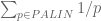
But he doesn’t compute the value to which the sum converges.

Your task is to compute the infinite sum. When you are finished, you are welcome to read a suggested solution, or to post your own solution or discuss the exercise in the comments below.

Pages: 1 2

Today’s exercise is from a beginner programming web site:

A prime number, such as 127, has no factors other than itself and one. A palindrome, such as 121, is the same number when its digits are reversed. A prime palindrome, such as 131, is both prime and a palindrome. Find the 100th prime palindrome.

Your task is to write a program to find the 100th prime palindrome; answer the question as if you were explaining the task to a beginner programmer. When you are finished, you are welcome to read or run a suggested solution, or to post your own solution or discuss the exercise in the comments below.

Pages: 1 2

[ I’ve had a couple of readers ask where I have been. I put in my retirement papers at work a few months ago, and will retire at the end of 2021. That sounds good, but setting up my post-retirement finances, learning about Medicare (it’s a huge mess) and deciding what to do with the rest of my life has been exhausting, and I still have a job to do. Here’s a simple exercise; I’ll try to be more regular about posting in future weeks. — Phil ]

Your task is to write a program to generate Motzkin Numbers (A001006). If you don’t like Motzkin numbers, pick any other sequence from the OEIS. When you are finished, you are welcome to read or run a suggested solution, or to post your own solution or discuss the exercise in the comments below.

Pages: 1 2

Aronson’s sequence 1, 4, 11, 16, 24, 29, 33, 35, 39, … (A005224) is an infinite self-referential sequence defined as:

T is the first, fourth, eleventh, … letter in this sentence.

Your task is to write a program that generates Aronson’s sequence and use it to compute the first hundred members of the sequence. When you are finished, you are welcome to read or run a suggested solution, or to post your own solution or discuss the exercise in the comments below.

Pages: 1 2

Cardinal numbers are those used for counting; spelled in letters, they are one, two, three, four, and so on.

Ordinal numbers are those used for ranking: spelled in letters, they are first, second, third, fourth, and so on.

Your task is to write a program that takes a number and returns the spelled-out cardinal and ordinal forms of that number. When you are finished, you are welcome to read or run a suggested solution, or to post your own solution or discuss the exercise in the comments below.

Pages: 1 2

Lagarias and Sloane study the “approximate squaring” map f(x) = x⌈x⌉ and its behavior when iterated in this paper.

Consider the fraction x = n / d when n > d > 1; let’s take 8/7 as an example. In the first step, the smallest integer greater than 8/7 (the “ceiling”) is 2, and 8/7 × 2 = 16/7. In the second step, the ceiling of 16/7 is 3, so we have 16/7 × 3 = 48/7. And in the third step, the ceiling of 48/7 is 7, so we have 48/7 × 7 = 48. Now the denominator is 1 and the result is an integer, so iteration stops, and we say that 8/7 goes to 48 in 3 steps.

Study shows the iteration is chaotic; sometimes the iteration stops in just a few steps, as in 8/7, sometimes it takes longer (6/5 goes to a number with 57735 digits in 18 steps), and sometimes it’s just ridiculous (200/199 goes to a number with 10⁴³⁵ digits). It is conjectured but not proven that iterated approximate squaring always terminates in an integer.

Your task is to write a program that iterates approximate squaring. When you are finished, you are welcome to read or run a suggested solution, or to post your own solution or discuss the exercise in the comments below.

Pages: 1 2

I had an email from a reader who found my factoring program on Stack Overflow:

Python 2.7.13 (default, Mar 13 2017, 20:56:15)
[GCC 5.4.0] on cygwin
Type "help", "copyright", "credits" or "license" for more information.
>>> def isPrime(n, k=5): # miller-rabin
...     from random import randint
...     if n < 2: return False
...     for p in [2,3,5,7,11,13,17,19,23,29]:
...         if n % p == 0: return n == p
...     s, d = 0, n-1
...     while d % 2 == 0:
...         s, d = s+1, d/2
...     for i in range(k):
...         x = pow(randint(2, n-1), d, n)
...         if x == 1 or x == n-1: continue
...         for r in range(1, s):
...             x = (x * x) % n
...             if x == 1: return False
...             if x == n-1: break
...         else: return False
...     return True
...
>>> def factors(n, b2=-1, b1=10000): # 2,3,5-wheel, then rho
...     def gcd(a,b): # euclid's algorithm
...         if b == 0: return a
...         return gcd(b, a%b)
...     def insertSorted(x, xs): # linear search
...         i, ln = 0, len(xs)
...         while i < ln and xs[i] < x: i += 1
...         xs.insert(i,x)
...         return xs
...     if -1 <= n <= 1: return [n]
...     if n < -1: return [-1] + factors(-n)
...     wheel = [1,2,2,4,2,4,2,4,6,2,6]
...     w, f, fs = 0, 2, []
...     while f*f <= n and f < b1:
...         while n % f == 0:
...             fs.append(f)
...             n /= f
...         f, w = f + wheel[w], w+1
...         if w == 11: w = 3
...     if n == 1: return fs
...     h, t, g, c = 1, 1, 1, 1
...     while not isPrime(n):
...         while b2 <> 0 and g == 1:
...             h = (h*h+c)%n # the hare runs
...             h = (h*h+c)%n # twice as fast
...             t = (t*t+c)%n # as the tortoise
...             g = gcd(t-h, n); b2 -= 1
...         if b2 == 0: return fs
...         if isPrime(g):
...             while n % g == 0:
...                 fs = insertSorted(g, fs)
...                 n /= g
...         h, t, g, c = 1, 1, 1, c+1
...     return insertSorted(n, fs)

He complained that the program failed to factor the number 100011322432435545, entering an infinite loop instead of returning a list of factors.

Your task is to figure out what is wrong, and fix it. When you are finished, you are welcome to read or run a suggested solution, or to post your own solution or discuss the exercise in the comments below.

Pages: 1 2

Today’s exercise comes from one of those online code exercises, via Stack Overflow:

There is a machine that can fix all potholes along a road 3 units in length. A unit of road will be represented by a period in a string. For example, “…” is one section of road 3 units in length. Potholes are marked with an “X” in the road, and also count as 1 unit of length. The task is to take a road of length N and fix all potholes with the fewest possible sections repaired by the machine.

The city where I live needs one of those machines.

Here are some examples:

.X.          1
.X...X       2
XXX.XXXX     3
.X.XX.XX.X   3

Your task is to write a program that takes a string representing a road and returns the smallest number of fixes that will remove all the potholes. When you are finished, you are welcome to read or run a suggested solution, or to post your own solution or discuss the exercise in the comments below.

Pages: 1 2

Today’s exercise comes from Stack Overflow:

Given a number N and a set of numbers s = {s1, s2, …, sn} where s1 < s2 < … < sn < N, remove all multiples of {s1, s2, …, sn} from the range 1..N.

You should look at the original post on Stack Overflow. The poster gets the answer wrong (he excludes 3), he get the explanation of his wrong answer wrong (he excludes 10 as a multiple of 2), and his algorithm is odd, to say the least. I’m not making fun of him, but I see this kind of imprecision of thought all the time on the beginner-programmer discussion boards, and I can only think that he will struggle to have a successful programming career.

Your task is to write a program that removes multiples from a range, as described above. When you are finished, you are welcome to read or run a suggested solution, or to post your own solution or discuss the exercise in the comments below.

Pages: 1 2