Programming Praxis

Hendrik Lenstra devised the elliptic curve factorization algorithm in 1987, an algorithm that is simultaneously elegant and of immense practical importance. This exercise describes his original algorithm. With some algorithmic tweaks that we won’t discuss here, Lenstra’s algorithm is generally quick to find factors in the 20- to 25-digit range, slower to find factors in the 40-digit range, and ineffective if the factors are much larger than about 50 digits; at this writing, the largest factor found by the elliptic curve algorithm has 67 digits.

Lenstra’s elliptic curve factorization algorithm works by searching for a point on the elliptic pseudo-curve E_a,b (mod n), where n =pq, that exists modulo p but not modulo q, or vice versa. In the previous exercise, we searched for that point by picking an initial point and repeatedly adding it to multiples of itself until the elliptic algebra failed.

Instead of repeated addition, Lenstra speeds the search by borrowing from Pollard’s p-1 method the idea of searching over a large product of small integers. Pollard’s method uses the least common multiple of numerous small integers, but Lenstra instead uses a large factorial. For instance, if you multiply 10000! by a point on an elliptic pseudo-curve, you are likely to find a factor of a 50-digit number somewhere in the middle of the computation. But Lenstra’s method admits a continuation that Pollard’s lacks; if one elliptic curve fails, you can choose another and try again. Or you can also increase the multiplier; if you don’t find a factor with a limit of 10000! and 1000 curves, you can try again with a limit of 1000000! and 1000000 curves.

Of course, there are some details to fill in, and instead of computing 10000! and then performing the elliptic multiplication, the work is done in small steps, checking the elliptic algebra after each. Here is Lenstra’s original algorithm, searching a single curve to a given limit:

To get started, choose a parameter for the limit, choose a random pseudo-elliptic curve E_a,b (mod n) and choose a random point (x,y) on the curve. Calculate the discriminant d = 4a³ + 27b² of the curve; if d = 0, the curve has a cusp or is self-intersecting, so choose a different curve. Then you can check if you were lucky; if gcd(d,n) > 1, d is a factor, so report it and quit. But most often d and n are co-prime, and you must continue.

The main body of Lenstra’s algorithm is a double-nested loop starting with random point (x,y):

for each prime p less than the limit
    for as many times as the base-p integer logarithm of the limit
        calculate a new (x,y) on Ea,b (mod n) as p times the old (x,y)
        if the calculation fails, report the finding of a factor

If you find a factor, the loop exits early; if the loop finishes, you can either choose a different curve, or increase the limit, or quit and report failure.

The elliptic addition, doubling and multiplication functions from the prior exercise need to be modified to recognize an error of the elliptic algebra before it occurs. For instance, when adding two points, first compute the denominator of the slope x₁ − x₂, and check that it has an inverse by calculating gcd(x₁ − x₂,n) before computing the slope and determining the sum of the two points; if the gcd is 1, you can proceed to calculate the inverse, if it is n you have been horribly unlucky (the point you are calculating isn’t on either of the two true sub-curves of the pseudo-curve) and you must exit the loop with failure, but if the gcd is strictly between 1 and n, it is a factor of n, so you can report it and quit. You may wish to calculate the integer logarithm in the inner loop by multiplying an accumulating product times the base p during the loop, stopping the loop when the accumulator exceeds the limit. The calculation of the large factorial is implicit in the two loops.

It is hard to choose the limit and the number of curves. In his original paper, Lenstra gives a formula for calculating exactly the limit and the number of curves, but unfortunately, the formula relies on the factorization, which of course is not yet known; his formula does give him a good way to prove the time-complexity bound, however. There are several papers that examine the question, but specific advice must be based on the specific implementation. The only general advice we can give is that the limit and number of curves must increase as the number to be factored increases, using too big or too small a limit and number of curves will cost you time rather than save it, and you will have to experiment with your implementation to know what works for you. Be aware that there can be considerable variance in the time it takes to perform a factorization, depending on how the random number generator chooses the parameters of the search.

Lenstra’s algorithm, as given above, searches a single curve to a given limit. To make a complete factorization, you must arrange to call it repeatedly in the event of failure, and then check the result, which may itself be composite, calling Lenstra’s algorithm recursively until the factorization is complete. And any real implementation of Lenstra’s algorithm first uses some light-weight method, such as trial division by small primes or Pollard’s rho algorithm, to quickly reduce the scope of a factorization.

Your task is to write a function that factors integers using Lenstra’s algorithm. Use your function to find the factors of (10⁸¹-1)/9; you may wish to do a timing comparison with Pollard’s rho factorization function. When you are finished, you are welcome to read or run a suggested solution, or to post your solution or discuss the exercise in the comments below.

Pages: 1 2

In the previous exercise we wrote a small library of functions on elliptic curves. Today we will use elliptic curves to perform integer factorization. The material in this exercise is based on a discussion in the second edition of the book Introduction to Cryptography with Coding Theory by Wade Trappe and Lawrence C. Washington.

It is easiest to explain the algorithm by an example. Consider the factorization of the number n = pq = 2773. To factor n, we choose an elliptic curve at random, let’s say y² ≡ x³ + 4x + 4 (mod 2773), where the modulus is the number to be factored. Of course, this is not really an elliptic curve, because the modulus of a real elliptic curve must be prime in order for us to compute the modular inverse required to determine the slope of the line connecting two points on the curve. It is exactly that fact that the elliptic curve algorithm exploits.

Next we choose a point on the curve; in this case, the point P = (1,3) works fine. In practice, it is easier to choose the a parameter randomly on the range 0 ≤ a < n, let the point be (1,1), then the b parameter is just –a, but you can select the parameters any way you like as long as a, b, x and y are all on the range 0 ≤ a < n and the point (x,y) is on the curve.

Now we begin a series of elliptic additions. The point 2P is (1771,705). Next we try to calculate 3P, but fail. The line through the points 2P = (1771,705) and P = (1,3) is 705 – 3 divided by 1771 – 1, the rise over the run, but gcd(1770,2773) = 59, so we cannot invert 1770 to calculate the slope of the line. We have found a point that is not on the elliptic curve. Of course, that is exactly what we were trying to do; 59 is a factor of 2773 = 59 × 47.

By the Chinese remainder theorem, the curve y² ≡ x³ + 4x + 4 (mod 2773) can be regarded as a pair of elliptic curves, one with modulus 59 and the other with modulus 47. Point 3P exists with modulus 47 but not with modulus 59. That’s how elliptic curve factorization works, allowing us to isolate the factor 59.

So the basic elliptic curve factorization algorithm is to choose a random elliptic curve (actually, a pseudo-elliptic curve) modulo the number to be factored, and a random point on the curve, then repeatedly build up multiples of the random point until the elliptic arithmetic fails, at which point the factor can be identified. The algorithm described here is a vastly simplified form of elliptic curve factorization, and is intended to teach the basic concepts rather than create a useful program; we’ll soon see a better version of the algorithm.

Your task is to write a function that performs integer factorization using the elliptic curve algorithm described above. Use your function to calculate the factors of 455839. When you are finished, you are welcome to read or run a suggested solution, or to post your solution or discuss the exercise in the comments below.

Pages: 1 2

Elliptic curves are a mathematical oddity. Originally derived from elliptic integrals that measure the area under an ellipse, elliptic curves have relationships to algebra, geometry, and number theory. Elliptic curves featured in the proof of Fermat’s last theorem and are used today in integer factorization and cryptography. We’ll see applications of elliptic curves in future exercises; the task today is to work out the basic arithmetic of elliptic curves. The simple definition of an elliptic curve is that it provides all the solutions to a generalized cubic equation.

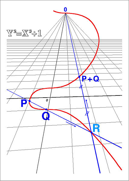
The standard form of an elliptic curve is y² = x³ + ax + b; we can also write E_a,b. Any formula that is cubic in two variables can be rewritten into this form via suitable transformations. In addition to the x,y points defined by the formula, an elliptic curve includes a “point at infinity,” denoted by ∞, analogous to an artist’s “vanishing point” that allows him to depict a three-dimensional image on a two-dimensional canvas. We will consider only elliptic curves where the discriminant 4a³ + 27b² is non-zero, meaning that the elliptic curve has no cusps or self-intersections.

The standard operation on an elliptic curve is the addition of two points, as shown in the diagram; this is, of course, different from vector addition of two points on a plane. Geometrically, points P and Q can be added by projecting a line between them and finding the “third point” R where the line intersects the curve, which is the negative of the point P + Q, as shown in the drawing by Jean Brette shown at right. Further, the point at infinity is the identity element for addition, so that P + ∞ = ∞ + P = P for any point P on an elliptic curve. Addition is both associative and commutative.

The addition law on elliptic curves is:

Given points P₁ = (x₁,y₁) and P₂ = (x₂,y₂), the point P₃ = (x₃,y₃) = P₁ + P₂, where points P₁, P₂ and P₃ lie on an elliptic curve y² = x³ + ax + b with non-zero discriminant 4a³ + 27b², can be calculated as

    x₃ = s² – x₁ – x₂

    y₃ = y₁ + s(x₃ – x₁)

where the slope s is

    s = (3x₁² + a) / (2y₁)

if P₁ = P₂ and

    s = (y₁ – y₂) / (x₁ – x₂)

otherwise.

The slope of the line connecting two points on an elliptic curve is calculated in the normal way, the difference in the rise divided by the difference in the run, except that if the two points are identical, the line “connecting” the two points is the tangent to the curve. Subtraction is addition of the negative, where the negative of (x,y) is (x,-y). Multiplication on an elliptic curve is just repeated addition, as it is with regular arithmetic.

We’ve been discussing elliptic curves over the real numbers, but the formulas work perfectly well on a finite field containing integers relative to a modulus. The division in the calculation of the slope is multiplication by the modular inverse, so the modulus must be prime. Our earlier exercise on modular arithmetic will be helpful.

A simple example may make things clear. Consider the elliptic curve y² ≡ x³ + 4x + 4 (mod 5). There are eight points on the curve: (0,2), (0,3), (1,2), (1,3), (2,0), (4,2), (4,3) and ∞; these points can be computed by substituting 0, 1, 2, 3 and 4 for x and computing the modular square root. Note that when x = 3 there are no solutions because 27 + 12 + 4 ≡ 43 ≡ 3 (mod 5) has no square roots, and when x = 2 there is only one solution, 8 + 8 + 4 ≡ 20 ≡ 0 (mod 5), and the square root of 0 is 0 regardless of the modulus. The sum of the points (1,2) and (4,3) is (4,2), the negative of the point (1,2) is (1,3), double the point (1,2) is (2,0), 3 times the point (1,2) is (1,3), 4 times the point (1,2) is ∞, and 5 times the point (1,2) is (1,2), whence the cycle repeats.

Your task is to write a library of functions for elliptic curves on a finite field. Your library should provide functions for addition, negation, subtraction, doubling, and multiplication; you may wish to represent a normal point as a triple (x y 1) and the point at infinity as the triple (0 1 0). When you are finished, you are welcome to read or run a suggested solution, or to post your solution or discuss the exercise in the comments below.

Pages: 1 2

Let’s Make A Deal! was a television game show that originated in the United States in the 1960s and has since been produced throughout the world. In one of the games, prizes were placed behind three doors, and the contestant was asked to pick a door; one door hid an automobile, the other two doors hid goats. Then the host, who knows what is behind the doors, opened one of the doors that the contestant did not pick, revealing in every case a goat, and asks if you want to switch doors. Is it to your advantage to switch your choice of doors?

Your task is to write a program that simulates a large number of games and determines whether or not it is to your advantage to switch doors. What are the odds that you will win the automobile by switching? When you are finished, you are welcome to read or run a suggested solution, or to post your solution or discuss the exercise in the comments below.

Pages: 1 2

Fermat’s little theorem states that for any prime number , and any other number , . Rearranging terms, we have , which means that divides the left-hand side of the equation, thus is a factor of the left-hand side.

John Pollard used this idea to develop a factoring method in 1974. His idea is to choose a very large number and see if it has any factors in common with , thus giving a factor of . A systematic way to test many very large numbers is by taking large factorials, which have many small factors within them. Thus, Pollard’s factorization algorithm is this:

1) Choose , which is known as the smoothness bound, and calculate the product of the primes to by .

2) Choose a random integer such that .

3) Calculate . If is strictly greater than 1, then it is a non-trivial factor of . Otherwise, continue to the next step.

4) Calculate . If , then is a non-trivial factor of . If , go to Step 1 and choose a larger . If , go back to Step 2 and choose another .

In Step 4, you can quit with failure instead of returning to Step 1 if becomes too large, where “too large” is probably somewhere around ; in that case, you will need to continue with some other factoring algorithm.

Your task is to write a function that factors integers by Pollard’s method. What are the factors of ? When you are finished, you are welcome to read or run a suggested solution, or to post your solution or discuss the exercise in the comments below.

Pages: 1 2

These three problems from the International Mathematical Olympiad recently popped up on the web.

IMO 1960 Problem 01

Determine all three-digit numbers N having the property that N is divisible by 11, and N/11 is equal to the sum of the squares of the digits of N.

IMO 1962 Problem 01

Find the smallest natural number n which has the following properties:

(a) Its decimal representation has 6 as the last digit.
(b) If the last digit 6 is erased and placed in front of the remaining digits, the resulting number is four times as large as the original number n.

IMO 1963 Problem 06

Five students, A,B,C,D,E, took part in a contest. One prediction was that the contestants would finish in the order ABCDE. This prediction was very poor. In fact no contestant finished in the position predicted, and no two contestants predicted to finish consecutively actually did so. A second prediction had the contestants finishing in the order DAECB. This prediction was better. Exactly two of the contestants finished in the places predicted, and two disjoint pairs of students predicted to finish consecutively actually did so. Determine the order in which the contestants finished.

Your task is to solve the three problems. When you are finished, you are welcome to read or run a suggested solution, or to post your solution or discuss the exercise in the comments below.

Pages: 1 2

Many newspapers publish a cryptogram each day; for instance:

P OYUUAOEXYW YM AEFGAD, FZGPEAG JAATUL, MYC ENA AGFOPEXYW PWG AWSYLVAWE YM ENA DPHHL ZCYICPVVAC

The deciphered cryptogram is usually a quote from a famous author, often advice for daily life or a pithy saying. Cryptographically, these puzzles are monoalphabetic substitution ciphers, with each of the twenty-six plain-text letters systematically replaced by a cipher-text letter.

Your task is to write a program that decrypts the daily cryptogram, and use that program to read the message given above. When you are finished, you are welcome to read or run a suggested solution, or to post your own solution or discuss the exercise in the comments below.

Pages: 1 2

I was helping my daughter with her math homework recently, and came across this problem in continued fractions:

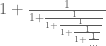
This fraction can be considered as a sequence of terms

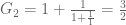
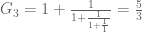
Or, in general

The first ten elements of the sequence are 1, 2, 3/2, 5/3, 8/5, 13/8, 21/13, 34/21, 55/34, and 89/55.

Your task is to write a program that evaluates the n^th element of the sequence. What is the value of ? When you are finished, you may read or run a suggested solution, or post your own solution or discuss the exercise in the comments below.

Pages: 1 2

Modular arithmetic is a branch of number theory that is useful in its own right and as a tool in such disciplines as integer factorization, calendrical and astronomical calculations, and cryptography. Modular arithmetic was systematized by Carl Friedrich Gauss in his book Disquisitiones Arithmeticae, published in 1801.

Modular arithmetic is a system of arithmetic for integers in which all results are expressed as non-negative integers less than the modulus. A familiar use of modular arithmetic is the twelve-hour clock, in which eight hours after nine o’clock is five o’clock; that is, 9 + 8 ≡ 5 (mod 12). The ≡ sign used in modular arithmetic specifies congruence, not equality. Two numbers are congruent in a given modulus if the difference between them is an even multiple of the modulus; for instance 17 ≡ 5 (mod 12). Modular addition is like regular addition, but “wraps around” at the modulus. Modular subtraction is the inverse operation of modular addition, and modular multiplication is just repeated modular addition; for instance 4 − 9 ≡ 7 (mod 12), and 3 × 7 ≡ 9 (mod 12).

Modular division is the inverse operation of modular multiplication, just as regular division is the inverse operation of regular multiplication. In modular arithmetic, the modular inverse of an integer p is that integer q for which p × q ≡ 1 (mod n); the modular inverse is undefined, just as division by zero is undefined, unless the target number is coprime to the modulus. The extended Euclidean algorithm calculates the inverse; given ax + by = g = gcd(x, y), when g = 1 and x > 0, b (mod x) and a (mod y) are the inverses of y (mod x) and x (mod y), respectively. Then modular division is just modular multiplication by the inverse. For instance, 9 ÷ 7 ≡ 3 (mod 12).

Exponentiation in modular arithmetic is repeated modular multiplication, just as exponentiation is repeated multiplication in normal arithmetic. Modular exponentiation could be performed by first computing the exponentiation and then performing the modulo operation, but that could involve a large intermediate result. A better method performs the modulo operations at each multiplication, squaring when possible to reduce the number of intermediate multiplications.

Square root is defined in modular arithmetic as that number which, when multiplied by itself, equals the target number, just as in normal arithmetic. And just as in normal arithmetic, every square root has a conjugate on the “other side” of zero, except that in modular arithmetic there is no “other side” of zero, so the two conjugates are the negatives of each other, adding to the modulus. For instance the square roots of 18 (mod 31) are 7 and 24, since 7 × 7 ≡ 18 (mod 31) and 24 × 24 ≡ 18 (mod 31), and 7 + 24 = 31.

Square root is a more difficult concept in modular arithmetic than regular arithmetic, because there are many cases where the modular square root does not exist. For instance, consider the squares x² (mod 13), 0 ≤ x < 13: 0, 1, 4, 9, 3, 12, 10, 10, 12, 3, 9, 4, 1. There is no number that can be squared modulo 13 to evaluate to 7, so the square root of 7 modulo 13 does not exist; the only numbers that have square roots modulo 13 are 1, 3, 4, 9, 10, and 12, or, equivalently, ±1, ±3, and ±4. Another restriction is that the modular square root is only defined if the modulus is an odd prime. For instance, consider the squares x² (mod 15), 0 ≤ x < 15: 0, 1, 4, 9, 1, 10, 6, 4, 4, 6, 10, 1, 9, 4, 1. The number 4 has two sets of conjugate square roots: ±2 and ±7. Since the solution is not unique, the modular square root can be said not to exist when the modulus is composite.

If you need a refresher on the math that supports modular arithmetic, you can look at any number theory textbook, or search the internet for terms such as modular arithmetic, bezout identity, modular inverse, jacobi symbol, and quadratic residue.

Your task is to write a library that provides convenient access to the basic operations of modular arithmetic: addition, subtraction, multiplication, division, exponentiation, and square root. When you are finished, you are welcome to read or run a suggested solution, or to post your own solution or discuss the exercise in the comments below.

Pages: 1 2